Statistical Rethinking - Exercises

2E1

Which of the expressions below correspond to the statement: the probability of rain on Monday?

1. \(Pr(rain)\)
2. \(\textbf{Pr(rain|Monday)}\)
3. \(Pr(Monday|rain)\)
4. \(\textbf{Pr(rain|Monday) / Pr(Monday)}\)

En página 36 se demuestra que la probabilidad conjunta de dos eventos es igual al numerador del teorema.

2E2

Which of the following expressions corresponds to the expression: \(Pr(Monday|rain)\)?

1. The probability of rain on Monday.
2. The probability of rain, given that it is Monday.
3. The probability of Monday, given that it is raining.
4. The probability that is Monday and it is raining.

2E3

Which of the expressions below correspond to the statement: the probability that it is Monday, given that it is raining?

1. \(\textbf{Pr(Monday|rain)}\)
2. \(Pr(rain|Monday)\)
3. \(Pr(rain|Monday)Pr(Monday)\)
4. \(\textbf{Pr(rain|Monday)Pr(Monday)/Pr(rain)}\)
5. \(Pr(Monday|rain)Pr(rain)/Pr(Monday)\)

2E4

The Bayesian statistician Bruno de Finetti (1906–1985) began his book on probability theory with the declaration: “PROBABILITY DOES NOT EXIST.” e capitals appeared in the original, so I imagine de Finetti wanted us to shout this statement. What he meant is that probability is a device for describing uncertainty from the perspective of an observer with limited knowledge; it has no objective reality. Discuss the globe tossing example from the chapter, in light of this statement. What does it mean to say “the probability of water is 0.7”?

La probabilidad es sólo un modelo en “small world”, y nos permite formalizar y modelar nuestra incertidumbre y así hacer inferencias (y reducirla con información proveniente de observaciones) tomándolo en cuenta; no obstante, no tenemos acceso al estado real del mundo y nos tendremos que limitar a nuestro conocimiento y el modelo.

2M1

Recall the globe tossing model from the chapter. Compute and plot the grid approximate posterior distribution for each of the following sets of observations. In each case, assume a uniform prior for \(p\).

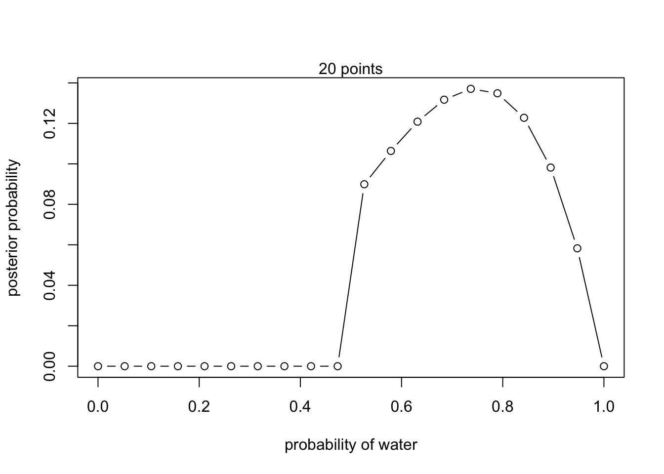
1. W,W,W

# define grid
p_grid <- seq(from = 0 , to = 1 , length.out = 20 )

# define prior
prior <- rep(1 , 20)

# compute likelihood at each value in grid
(likelihood <- dbinom(3, size = 3 , prob = p_grid))

##  [1] 0.0000000000 0.0001457938 0.0011663508 0.0039364339 0.0093308062
##  [6] 0.0182242309 0.0314914711 0.0500072897 0.0746464499 0.1062837148
## [11] 0.1457938475 0.1940516110 0.2519317685 0.3203090830 0.4000583175
## [16] 0.4920542353 0.5971715994 0.7162851728 0.8502697186 1.0000000000

# compute product of likelihood and prior
(unstd.posterior <- likelihood * prior)

##  [1] 0.0000000000 0.0001457938 0.0011663508 0.0039364339 0.0093308062
##  [6] 0.0182242309 0.0314914711 0.0500072897 0.0746464499 0.1062837148
## [11] 0.1457938475 0.1940516110 0.2519317685 0.3203090830 0.4000583175
## [16] 0.4920542353 0.5971715994 0.7162851728 0.8502697186 1.0000000000

# standardize the posterior, so it sums to 1
(posterior <- unstd.posterior / sum(unstd.posterior))

##  [1] 0.000000e+00 2.770083e-05 2.216066e-04 7.479224e-04 1.772853e-03
##  [6] 3.462604e-03 5.983380e-03 9.501385e-03 1.418283e-02 2.019391e-02
## [11] 2.770083e-02 3.686981e-02 4.786704e-02 6.085873e-02 7.601108e-02
## [16] 9.349030e-02 1.134626e-01 1.360942e-01 1.615512e-01 1.900000e-01

## Plot
plot( p_grid , posterior , type = "b" ,
    xlab = "probability of water" , ylab = "posterior probability")
mtext("20 points")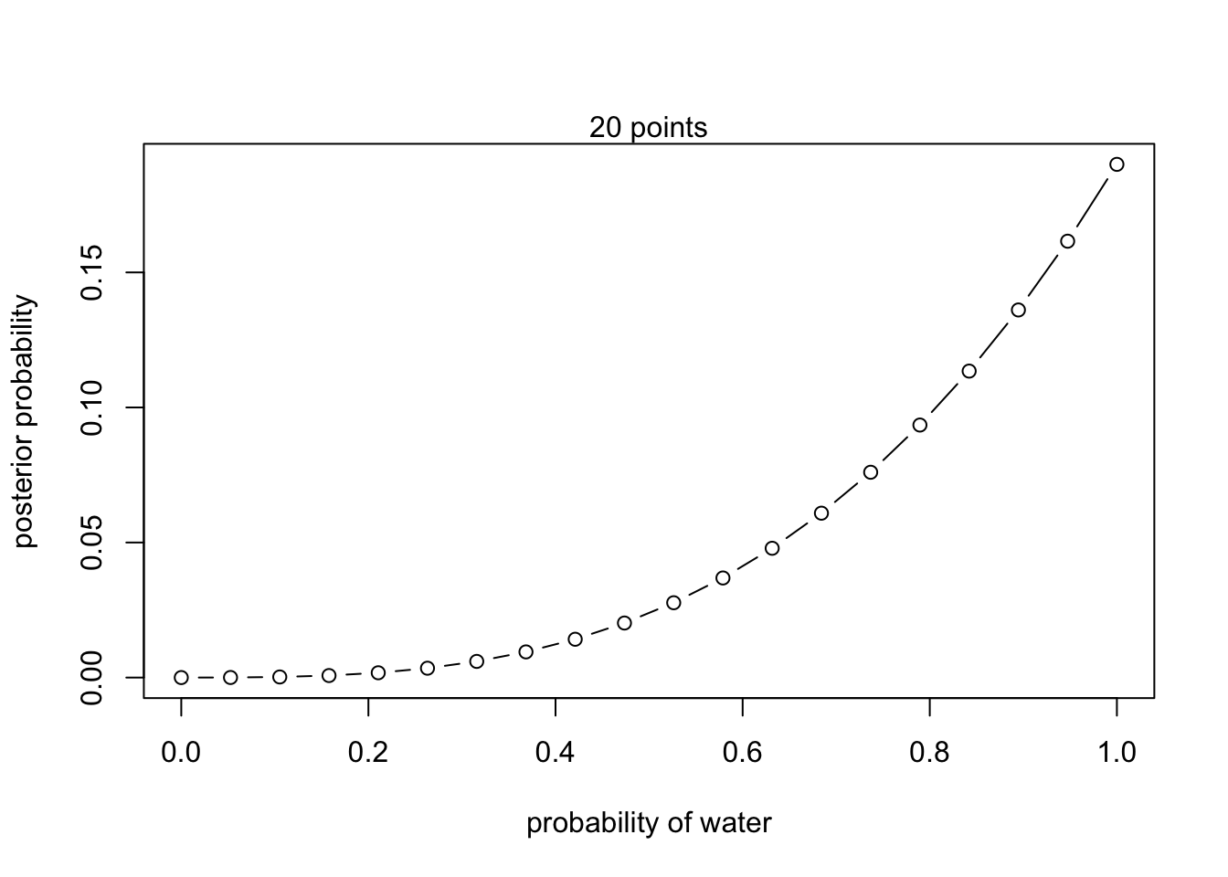

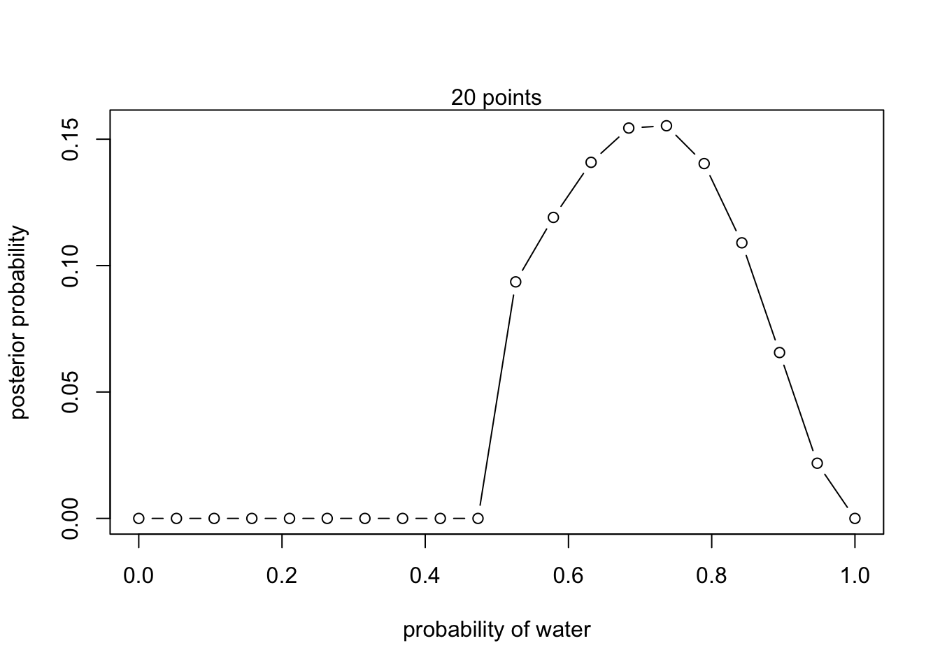
2. W,W,W,L

# define grid
p_grid <- seq(from = 0 , to = 1 , length.out = 20 )

# define prior
prior <- rep(1 , 20)

# compute likelihood at each value in grid
(likelihood <- dbinom(3, size = 4 , prob = p_grid))

##  [1] 0.0000000000 0.0005524819 0.0041743081 0.0132595668 0.0294657039
##  [6] 0.0537135228 0.0861871840 0.1263342055 0.1728654630 0.2237551891
## [11] 0.2762409742 0.3268237659 0.3712678693 0.4046009469 0.4211140185
## [16] 0.4143614613 0.3771610101 0.3015937570 0.1790041513 0.0000000000

# compute product of likelihood and prior
(unstd.posterior <- likelihood * prior)

##  [1] 0.0000000000 0.0005524819 0.0041743081 0.0132595668 0.0294657039
##  [6] 0.0537135228 0.0861871840 0.1263342055 0.1728654630 0.2237551891
## [11] 0.2762409742 0.3268237659 0.3712678693 0.4046009469 0.4211140185
## [16] 0.4143614613 0.3771610101 0.3015937570 0.1790041513 0.0000000000

# standardize the posterior, so it sums to 1
(posterior <- unstd.posterior / sum(unstd.posterior))

##  [1] 0.0000000000 0.0001460636 0.0011035915 0.0035055261 0.0077900579
##  [6] 0.0142006265 0.0227859195 0.0333998734 0.0457016732 0.0591557525
## [11] 0.0730317932 0.0864047260 0.0981547300 0.1069672331 0.1113329114
## [16] 0.1095476898 0.0997127416 0.0797344889 0.0473246020 0.0000000000

## Plot
plot( p_grid , posterior , type = "b" ,
    xlab = "probability of water" , ylab = "posterior probability")
mtext("20 points")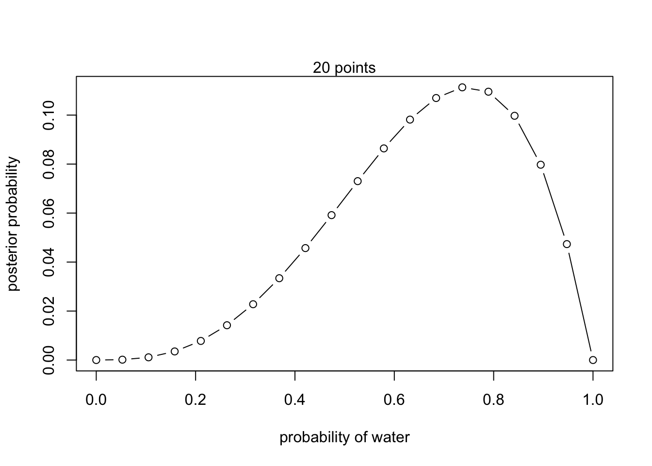

3. L,W,W,L,W,W,W

# define grid
p_grid <- seq(from = 0 , to = 1 , length.out = 20 )

# define prior
prior <- rep(1 , 20)

# compute likelihood at each value in grid
(likelihood <- dbinom(5, size = 7 , prob = p_grid))

##  [1] 0.000000e+00 7.611830e-06 2.172661e-04 1.461471e-03 5.412857e-03
##  [6] 1.438965e-02 3.087358e-02 5.685868e-02 9.314926e-02 1.387256e-01
## [11] 1.902958e-01 2.421517e-01 2.864484e-01 3.140244e-01 3.158816e-01
## [16] 2.854436e-01 2.217106e-01 1.334285e-01 4.439219e-02 0.000000e+00

# compute product of likelihood and prior
(unstd.posterior <- likelihood * prior)

##  [1] 0.000000e+00 7.611830e-06 2.172661e-04 1.461471e-03 5.412857e-03
##  [6] 1.438965e-02 3.087358e-02 5.685868e-02 9.314926e-02 1.387256e-01
## [11] 1.902958e-01 2.421517e-01 2.864484e-01 3.140244e-01 3.158816e-01
## [16] 2.854436e-01 2.217106e-01 1.334285e-01 4.439219e-02 0.000000e+00

# standardize the posterior, so it sums to 1
(posterior <- unstd.posterior / sum(unstd.posterior))

##  [1] 0.000000e+00 3.205153e-06 9.148535e-05 6.153894e-04 2.279220e-03
##  [6] 6.059124e-03 1.300010e-02 2.394178e-02 3.922284e-02 5.841391e-02
## [11] 8.012882e-02 1.019641e-01 1.206163e-01 1.322279e-01 1.330099e-01
## [16] 1.201932e-01 9.335685e-02 5.618344e-02 1.869245e-02 0.000000e+00

## Plot
plot( p_grid , posterior , type = "b" ,
    xlab = "probability of water" , ylab = "posterior probability")
mtext("20 points")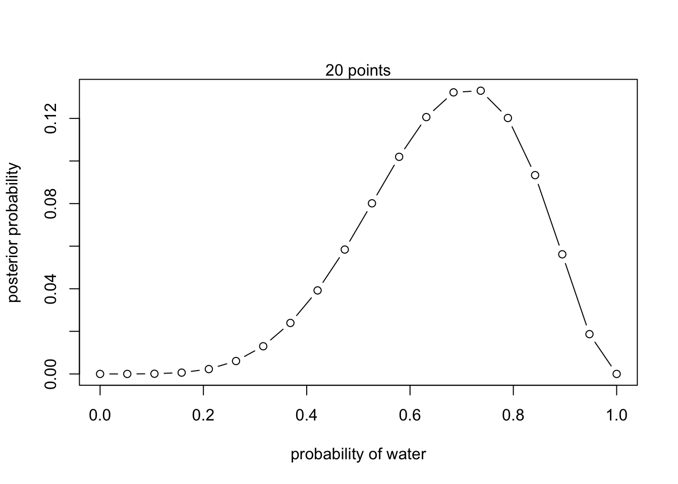

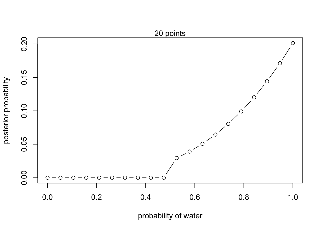
2M2

Now assume a prior for \(p\) that is equal to zero when \(p < 0.5\) and is a positive constant when \(p ≥ 0.5\). Again compute and plot the grid approximate posterior distribution for each of the sets of observations in the problem just above.

# New prior
prior <- ifelse( p_grid < 0.5 , 0 , 1 )

1. W,W,W

2. W,W,W,L

3. L,W,W,L,W,W,W

2M3

Suppose there are two globes, one for Earth and one for Mars. e Earth globe is 70% covered in water. e Mars globe is 100% land. Further suppose that one of these globes—you don’t know which—was tossed in the air and produced a “land” observation. Assume that each globe was equally likely to be tossed. Show that the posterior probability that the globe was the Earth, conditional on seeing “land” (\(Pr(Earth|land)\)), is 0.23.

\[Pr(Earth|Land) = \frac{Pr(Land|Earth) P(Earth)}{Pr(Land|Earth) P(Earth) + Pr(Land|Mars) P(Mars)} = \frac{.3 \times .5}{.3 \times .5 + 1 \times .5}\]

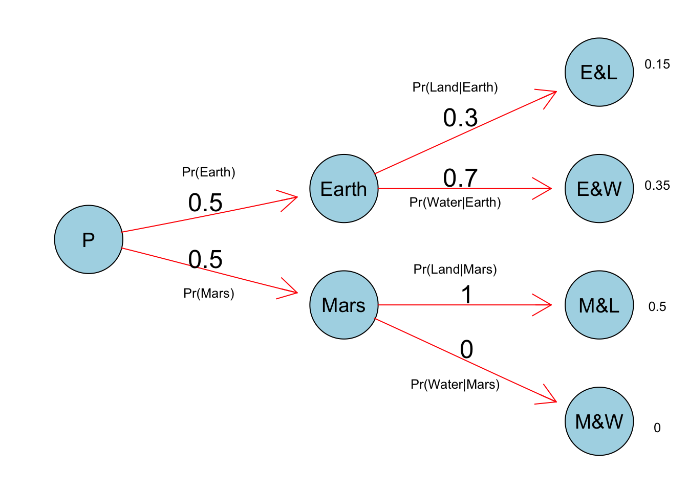
pr_E = .5 # Pr(Earth)
pr_M = .5 # Pr(Mars)

pr_L_E = .3 # Pr(Land|Earth)
pr_L_M = 1 # Pr(land|Mars)

pr_L = pr_L_E * pr_E + pr_L_M * pr_M # Pr(Land)

# Pr(Earth|land)
(pr_E_L = (pr_L_E * pr_E) / pr_L)

## [1] 0.2307692

2M4

Suppose you have a deck with only three cards. Each card has two sides, and each side is either black or white. One card has two black sides. e second card has one black and one white side. e third card has two white sides. Now suppose all three cards are placed in a bag and shu ed. Someone reaches into the bag and pulls out a card and places it at on a table. A black side is shown facing up, but you don’t know the color of the side facing down. Show that the probability that the other side is also black is 2/3. Use the counting method (Section 2 of the chapter) to approach this problem. is means counting up the ways that each card could produce the observed data (a black side facing up on the table).

2M5

Now suppose there are four cards: B/B, B/W, W/W, and another B/B. Again suppose a card is drawn from the bag and a black side appears face up. Again calculate the probability that the other side is black.

2M6

Imagine that black ink is heavy, and so cards with black sides are heavier than cards with white sides. As a result, it’s less likely that a card with black sides is pulled from the bag. So again assume there are three cards: B/B, B/W, and W/W. A er experimenting a number of times, you conclude that for every way to pull the B/B card from the bag, there are 2 ways to pull the B/W card and 3 ways to pull the W/W card. Again suppose that a card is pulled and a black side appears face up. Show that the probability the other side is black is now 0.5. Use the counting method, as before.

2M7

Assume again the original card problem, with a single card showing a black side face up. Before looking at the other side, we draw another card from the bag and lay it face up on the table. The face that is shown on the new card is white. Show that the probability that the rst card, the one showing a black side, has black on its other side is now 0.75. Use the counting method, if you can. Hint: Treat this like the sequence of globe tosses, counting all the ways to see each observation, for each possible rst card.

2H1

Suppose there are two species of panda bear. Both are equally common in the wild and live in the same places. ey look exactly alike and eat the same food, and there is yet no genetic assay capable of telling them apart. ey di er however in their family sizes. Species A gives birth to twins 10% of the time, otherwise birthing a single infant. Species B births twins 20% of the time, otherwise birthing singleton infants. Assume these numbers are known with certainty, from many years of eld research.

Now suppose you are managing a captive panda breeding program. You have a new female panda of unknown species, and she has just given birth to twins. What is the probability that her next birth will also be twins?

2H2

Recall all the facts from the problem above. Now compute the probability that the panda we have is from species A, assuming we have observed only the first birth and that it was twins.

2H3

Continuing on from the previous problem, suppose the same panda mother has a second birth and that it is not twins, but a singleton infant. Compute the posterior probability that this panda is species A.

2H4

A common boast of Bayesian statisticians is that Bayesian inference makes it easy to use all of the data, even if the data are of di erent types.

So suppose now that a veterinarian comes along who has a new genetic test that she claims can identify the species of our mother panda. But the test, like all tests, is imperfect. is is the informa- tion you have about the test:

• The probability it correctly identifies a species A panda is 0.8.
• The probability it correctly identifies a species B panda is 0.65.

The vet administers the test to your panda and tells you that the test is positive for species A. First ignore your previous information from the births and compute the posterior probability that your panda is species A. en redo your calculation, now using the birth data as well.

3E1

How much posterior probability lies below \(p\) = 0.2?

3E2

How much posterior probability lies above \(p\) = 0.8?

3E3

How much posterior probability lies between \(p\) = 0.2 and \(p\) = 0.8?

3E4

20% of the posterior probability lies below which value of \(p\)?

3E5

20% of the posterior probability lies above which value of \(p\)?

3E6

Which values of \(p\) contain the narrowest interval equal to 66% of the posterior probability?

3E7

Which values of \(p\) contain 66% of the posterior probability, assuming equal posterior probability both below and above the interval?

3M1

Suppose the globe tossing data had turned out to be 8 water in 15 tosses. Construct the posterior distribution, using grid approximation. Use the same at prior as before.

3M2

Draw 10,000 samples from the grid approximation from above. en use the samples to calculate the 90% HPDI for \(p\).

3M3

Construct a posterior predictive check for this model and data. is means simulate the distri- bution of samples, averaging over the posterior uncertainty in \(p\). What is the probability of observing 8 water in 15 tosses?

3M4

Using the posterior distribution constructed from the new (8/15) data, now calculate the probability of observing 6 water in 9 tosses.

3M5

Start over at 3M1, but now use a prior that is zero below \(p\) = 0.5 and a constant above \(p\) = 0.5. is corresponds to prior information that a majority of the Earth’s surface is water. Repeat each problem above and compare the inferences. What di erence does the better prior make? If it helps, compare inferences (using both priors) to the true value \(p\) = 0.7.

3H1

Using grid approximation, compute the posterior distribution for the probability of a birth being a boy. Assume a uniform prior probability. Which parameter value maximizes the posterior probability?

3H2

Using the sample function, draw 10,000 random parameter values from the posterior distribution you calculated above. Use these samples to estimate the 50%, 89%, and 97% highest posterior density intervals.

3H3

Use rbinom to simulate 10,000 replicates of 200 births. You should end up with 10,000 numbers, each one a count of boys out of 200 births. Compare the distribution of predicted numbers of boys to the actual count in the data (111 boys out of 200 births). There are many good ways to visualize the simulations, but the dens command (part of the rethinking package) is probably the easiest way in this case. Does it look like the model ts the data well? at is, does the distribution of predictions include the actual observation as a central, likely outcome?

3H4

Now compare 10,000 counts of boys from 100 simulated first borns only to the number of boys in the first births, birth1. How does the model look in this light?

3H5

The model assumes that sex of first and second births are independent. To check this assump- tion, focus now on second births that followed female first borns. Compare 10,000 simulated counts of boys to only those second births that followed girls. To do this correctly, you need to count the number of first borns who were girls and simulate that many births, 10,000 times. Compare the counts of boys in your simulations to the actual observed count of boys following girls. How does the model look in this light? Any guesses what is going on in these data?

4E1

In the model definition below, which line is the likelihood?

\[y_i \sim Normal(\mu, \sigma)\] \[\mu \sim Normal(0, 10)\] \[\sigma \sim Uniform(0, 0)\]

4E2

In the model de definition just above, how many parameters are in the posterior distribution?

4E3

Using the model de definition above, write down the appropriate form of Bayes’ theorem that includes the proper likelihood and priors.

4E4

In the model de definition below, which line is the linear model?

\[y_i \sim Normal(\mu, \sigma)\] \[\mu = \alpha + \beta x_i\] \[\alpha \sim Normal(0, 10)\] \[\beta \sim Normal(0,1)\] \[\sigma \sim Uniform(0, 10)\]

4E5

In the model de definition just above, how many parameters are in the posterior distribution?

4M1

For the model de definition below, simulate observed heights from the prior (not the posterior)

\[y_i \sim Normal(\mu, \sigma)\] \[\mu \sim Normal(0, 10)\] \[\sigma \sim Uniform(0, 10)\]

4M2

Translate the model just above into a map formula.

4M3

Translate the map model formula below into a mathematical model de definition.

flist <- alist(
    y ~ dnorm( mu , sigma ),
    mu <- a + b*x,
    a ~ dnorm( 0 , 50 ),
    b ~ dunif( 0 , 10 ),
    sigma ~ dunif( 0 , 50 )
)

4M4

A sample of students is measured for heigh teach year for 3years. After the third year, you want to fit a linear regression predicting height using year as a predictor. Write down the mathematical model definition for this regression, using any variable names and priors you choose. Be prepared to defend your choice of priors.

4M5

Now suppose I tell you that the average height in the first year was 120 cm and that every student got taller each year. Does this information lead you to change your choice of priors? How?

4M6

Now suppose I tell you that the variance among heights for students of the same age is never more than 64cm. How does this lead you to revise your priors?

4H1

The weights listed below were recorded in the !Kung census, but heights were not recorded for these individuals. Provide predicted heights and 89% intervals (either HPDI or PI) for each of these individuals. That is, fill in the table below, using model-based predictions.

4H2

Select out all the rows in the Howell1 data with ages below 18 years of age. If you do it right, you should end up with a new data frame with 192 rows in it.

1. Fit a linear regression to these data, using map. Present and interpret the estimates. For every 10 units of increase in weight, how much taller does the model predict a child gets?

2. Plot the raw data, with height on the vertical axis and weight on the horizontal axis. Super-impose the MAP regression line and 89% HPDI for the mean. Also superimpose the 89% HPDI for predicted heights.

3. What aspects of the model fit concern you? Describe the kinds of assumptions you would change, if any, to improve the model. You don’t have to write any new code. Just explain what the model appears to be doing a bad job of, and what you hypothesize would be a better model.

4H3

Suppose a colleague of yours, who works on allometry, glances at the practice problems just above. Your colleague exclaims, “That’s silly. Everyone knows that it’s only the logarithm of body weight that scales with height!” Let’s take your colleague’s advice and see what happens.

1. Model the relationship between height (cm) and the natural logarithm of weight (log-kg). Use the entire Howell1 data frame, all 544 rows, adults and non-adults. Fit this model, using quadratic approximation:

\[h_i \sim Normal(\mu, \sigma)\] \[\mu_i = \alpha + \beta log(w_i)\] \[\alpha \sim Normal(178, 100)\] \[\beta \sim Normal(0, 100)\] \[\sigma \sim Uniform(0, 50)\]

where \(h_i\) is the height of individual \(i\) and \(w_i\) is the weight (in kg) of individual \(i\). The function for computing a natural log in R is just log. Can you interpret the resulting estimates?

2. Begin with this plot:

 plot(height ~ weight, data = Howell1,
    col = col.alpha(rangi2, 0.4)

Then use samples from the quadratic approximate posterior of the model in (a) to superimpose on the plot: (1) the predicted mean height as a function of weight, (2) the 97% HPDI for the mean, and (3) the 97% HPDI for predicted heights.